Adding Ion Fields
In addition to being able to create absorption spectra, Trident can be used to calculate the ionization states for different metal species present in different thermodynamic states of the CGM and IGM. There are several tools you can use to access this functionality. You can simply obtain ion fractions as a function of density, temperature, and redshift, or you can postprocess whole simulation outputs to add fields for ions not explicitly tracked in the simulation. These can later be analyzed using the standard yt analysis packages. This page provides some examples on how to utilize this functionality.
How does it work?
When you installed Trident, you were forced to download an ion table, a
data table consisting of dimensions in density, temperature, and redshift.
This ion table was constructed by running many independent Cloudy instances
to approximate the ionization states of all ionic species of the first 30
elements. The ionic species were calculated assuming collisional
ionization equilibrium based on different density and
temperature values and photoionization from a metagalactic ultraviolet
background unique to each ion table. The currently preferred ion table
uses the Haardt Madau 2012 model. You can change your default
ionization model by changing your config file (see: Manually Installing your Ionization Table), or
by specifying it directly in the ionization_table keywords of the following
functions.
By following the process below, you will add different ion fields to your dataset based on the above assumptions using the dataset’s redshift, and the values of density, temperature, and metallicity found for each gas parcel in your dataset.
Calculating ion fractions
In its simplest form, one may wish to calculate a single (or multiple) ion fraction
for some arbitrary ion as a function of the thermodynamic properties of the gas.
This can be calculated without any simulation dataset output at all, simply by
linearly interpolating over the ion table referenced above. This is best achieved
using the function calculate_ion_fraction. In the
following example, we’ll calculate the fraction of magnesium that is in its 1st
ionized state (Mg II) for gas at two densities and temperatures at redshift 0:
import trident
density = [1e-2, 1e-4] # as n_H in cm**-3
temperature = [1e4, 1e6] # in K
redshift = [0, 0]
trident.calculate_ion_fraction('Mg II', density, temperature, redshift)
[5.30884437e-01 1.00000000e-30]
The result indicates that Mg II is a dominant ion of magnesium in cool dense gas, whereas it is totally absent in hot, tenuous gas.
Generating species fields
One may wish to post-process an entire dataset to include the ion information for some arbitrary ion as an additional scalar field that can be accessed by yt. As always, we first need to import yt and Trident and then we load up a dataset:
import yt
import trident
fn = 'enzo_cosmology_plus/RD0009/RD0009'
ds = yt.load(fn)
To add ion fields we use the add_ion_fields function. This
will add fields for whatever ions we specify in the form of:
Ion fraction field. e.g.
Mg_p1_ion_fractionNumber density field. e.g.
Mg_p1_number_densityDensity field. e.g.
Mg_p1_densityMass field. e.g.
Mg_p1_mass
Note
Trident follows yt’s naming convention
for atomic, molecular, and ionic species fields. In short, the ionic
prefix consists of the element and the number of times ionized it is:
e.g. H I = H_p0, Mg II = Mg_p1, O VI = O_p5 (p is for plus).
Let’s add fields for O VI (five-times-ionized oxygen):
trident.add_ion_fields(ds, ions=['O VI'])
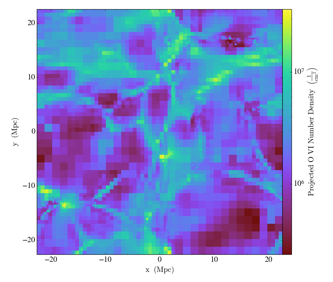
To show how one can use this newly generated field, we’ll make a projection of the O VI number density field to show its column density map:
proj = yt.ProjectionPlot(ds, "z", "O_p5_number_density")
proj.save()
which produces:
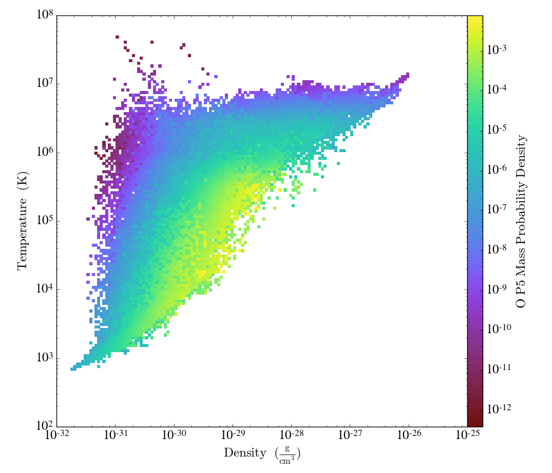
We can similarly create a phase plot to show where the O VI mass lives as a function of density and temperature:
# we need to create a data object from the dataset to make a phase plot
ad = ds.all_data()
phase = yt.PhasePlot(ad, "density", "temperature", ["O_p5_mass"],
                     weight_field="O_p5_mass", fractional=True)
phase.save()
resulting in: